DMI – Graduate Course in Computer Science
Copyleft
![]() 2016-2017 Giuseppe Scollo
2016-2017 Giuseppe Scollo
![]()
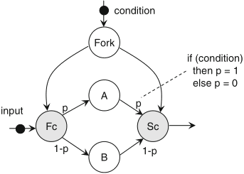
example: 4-level pulse-amplitude signal modulation (PAM-4)
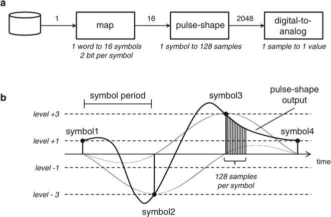
Schaumont, Figure 2.1 - (a) Pulse-amplitude modulation system. (b) Operation of the pulse-shaping unit
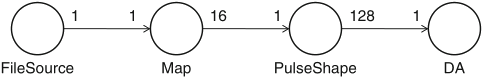
Schaumont, Figure 2.2 - Data flow model for the pulse-amplitude modulation system
a software model of the PAM-4 system is feasible, see for example the C program in Schaumont, Listing 2.1, where each block is represented as a function, yet:
in the model in figure, functions are represented by actors linked through communication channels modeled as FIFO queues
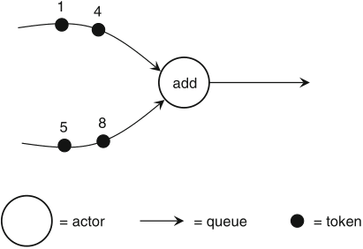
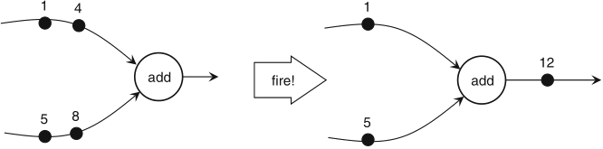
Schaumont, Figure 2.3 - Data flow model of an addition
actors are functional processing units with no internal state
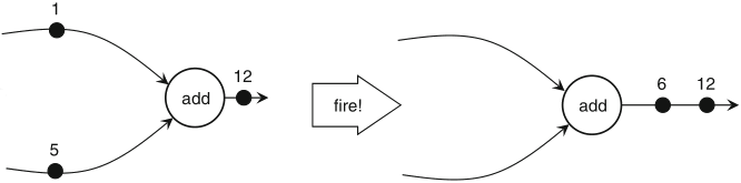
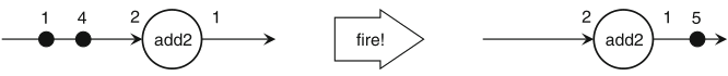
in multirate dataflow graphs each actor may consume more than one token on each input channel and may produce more than one token on each output channel, at every firing
graphs with fixed production and consumption rates are said synchronous dataflow graphs (SDF)
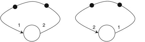
Schaumont, Figure 2.8 - SDF graphs are determinate
desirable properties of an SDF graph:
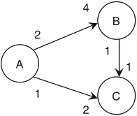
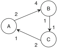
Schaumont, Figure 2.9 - Which SDF graph will deadlock, and which is unstable?
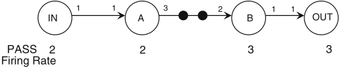
Schaumont, Figure 2.10 - Example SDF graph for PASS construction
PASS: periodic admissible sequential schedule
PASS construction algorithm, if one exists (Lee):
Schaumont, Figure 2.11 - A deadlocked graph
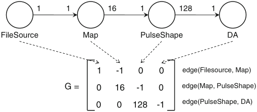
Schaumont, Figure 2.12 - Topology matrix for the PAM-4 system
application of the method by Lee:
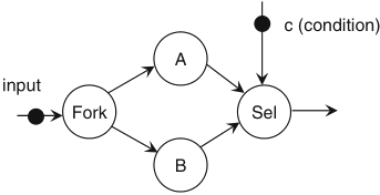
modeling control flow is not easy with SDF graphs...
a few problematic issues:
minimal extensions, preserving SDF semantics:
useful for performance analysis and to evaluate performance-enhancing transformations
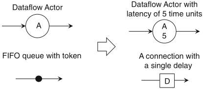
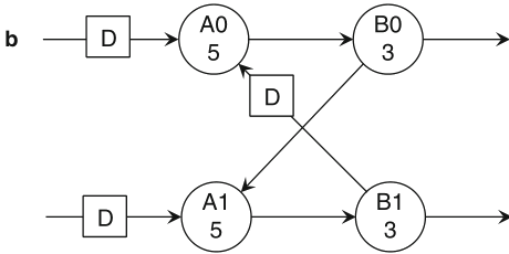
Schaumont, Figure 2.15 - Enhancing the SDF model with resources: execution time for actors, delays for FIFO queues
in the initial state, buffers always hold a token
a buffer may hold a token for the duration of a single activation of the next actor
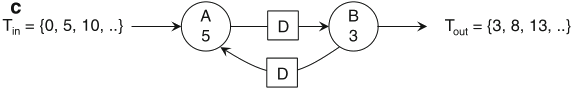
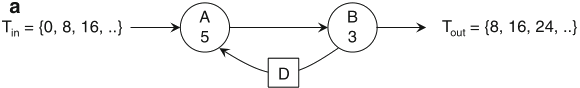
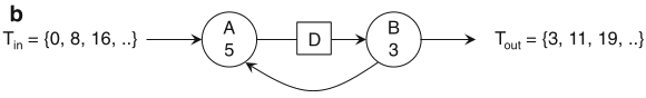
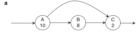
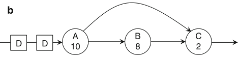
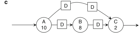
Schaumont, Figure 2.16 - Three data flow graphs
by adding buffers, pipelining may increase the throughput of an SDF graph
number and distribution of buffers in an SDF graph affect its throughput
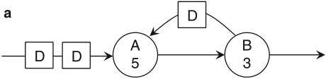
loops also affect its latency and throughput; two concepts to see this:
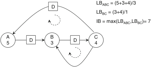
Schaumont, Figure 2.17 - Calculating loop bound and iteration bound
the throughput of an SDF graph cannot be higher than (the reciprocal of) its iteration bound

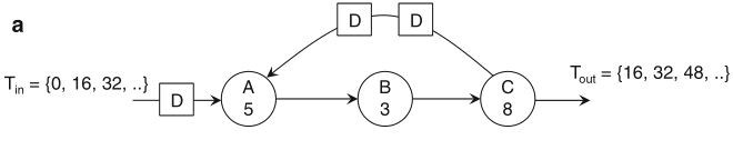
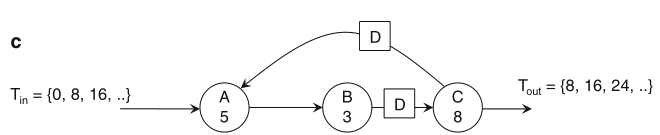
Schaumont, Figure 2.18 - Iteration bound for a linear graph
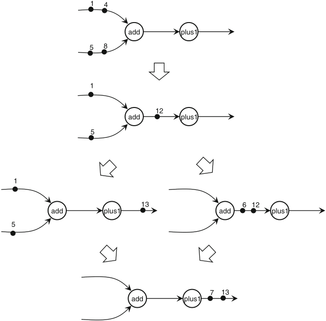
transformation of a multirate SDF graph to single-rate, in 5 steps:
this transformation redistributes the buffers without changing their total number

Schaumont, Figure 2.21
- Retiming: (a) Original Graph. (b) Graph after first re-timing transformation.
(c) Graph after second re-timing transformation
pipelining = additional buffers + retiming
Schaumont, Figure 2.22
- Pipelining: (a) Original graph. (b) Graph after adding two pipeline stages.
(c) Graph after retiming the pipeline stages
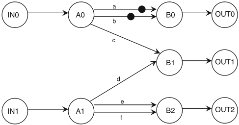
replication of a given SDF graph into several copies in order to increase the parallelism of input stream processing
the ν-unfolding of an SDF graph yields a graph with ν copies of each actor and of each edge
if edge AB connects actors A and B in the original graph, where it carries n buffers, then in the transformed graph, for i = 0..ν-1: